
Visualizing the Code Co-Occurrence Table
Sankey Diagram
Video Tutorial: Sankey Diagrams in ATLAS.ti Windows
Data Visualization is a great way to simplify the complexity of understanding relationships among data. The Sankey Diagram is one such powerful technique to visualize the association of data elements. Originally, Sankey diagrams were named after Irish Captain Matthew Henry Phineas Riall Sankey, who used this type of diagram in 1898 in a classic figure showing the energy efficiency of a steam engine. Today, Sankey diagrams are used for presenting data flows and data connections across various disciplines.
-
Sankey diagrams allow you to show complex processes visually, with a focus on a single aspect or resource that you want to highlight.
-
They offer the added benefit of supporting multiple viewing levels. Viewers can get a high level view, see specific details, or generate interactive views.
-
Sankey diagrams make dominant factors stand out, and they help you to see the relative magnitudes and/or areas with the largest contributions.
In ATLAS.ti, the Sankey diagram complements the Code Co-occurrence Table. As soon as you create a table, a Sankey diagram visualizing the data will be shown below the table.
Further Reading
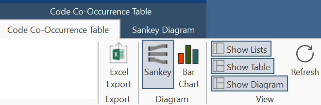
As soon as you create a table, a bar chart will be shown in the area below the table. To see a Sankey Diagram instead, click the Sankey button in the Diagram section of the ribbon.
If you need more space on your screen for the diagram, you can also deactivate the lists and/or the table in the ribbon.
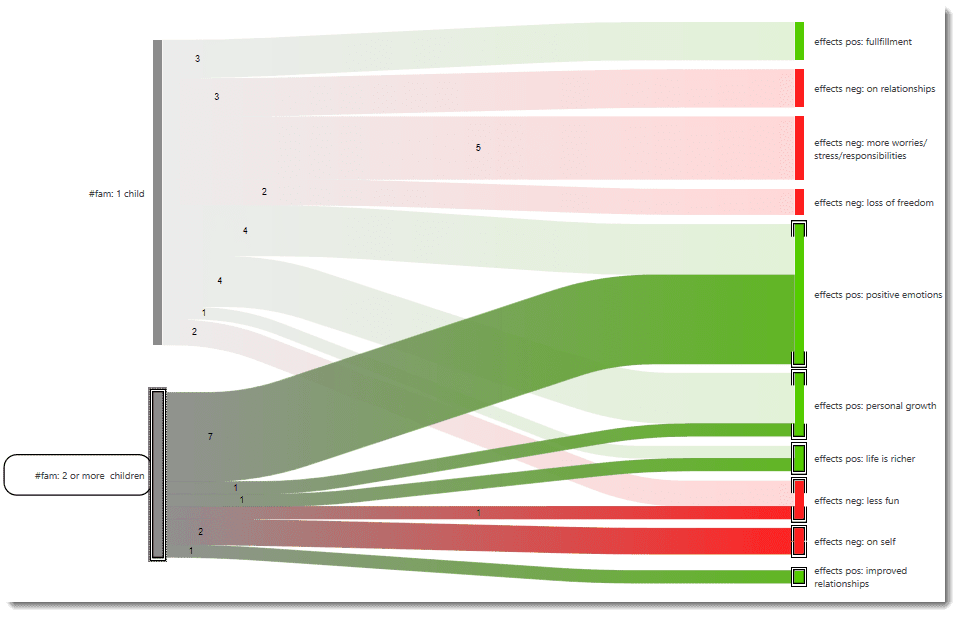
The row and column entities of the table are represented in the Sankey model as nodes and edges, showing the strength of co-occurrence between the pairs of nodes. In the Code Co-occurrence table, the connecting pairs are codes for both rows and columns.
Edge: For each table cell containing a value, an edge is displayed between the diagram nodes. The thickness of the edges resemble the cell values of the table. Cells with value 0 are not displayed in the Sankey view.
The key to reading and interpreting Sankey Diagrams is to remember that the width is proportional to the quantity represented.
Layout
The Sankey diagram, similar to the network editor, applies a layout for its nodes and consequently to the edges connecting nodes to create an easy to comprehend visualization of the data. This basic layout places the selected entities (nodes in Sankey terminology) into vertical „layers“ with the row entities placed to the left and the column entities to the right. If nodes have incoming as well as outgoing links in the currently visible set of nodes, they will be placed in intermediate lanes or layers.
In many situations, the initial layout already meets the researchers requirements. However, there are some options to modify the initial layout.
Swapping columns and rows for the table will also affect the Sankey diagram and result in a 180° rotation.
Interactivity
-
To display the quotations that are responsible for the co-occurrence of two entities, click on the connecting edge. This has the same effect as clicking a table cell. You see the quotations displayed in the Quotation Reader to the right.
-
If you hover over an edge, you see the number that is also displayed in the table cell, which are the number of times the pair of codes co-occur.
-
To support finding the correct link, moving the mouse highlights the hovered edges. After selecting an edge, the unselected edges are dimmed to further increase the visibility of the edge under consideration.
-
Selecting a node will highlight this node as well as all its incoming and outgoing edges. This makes it easy to spot areas of connectivity.
-
You can also use the nodes label for selection. This allows you to do a „single-handed“ multi-selection which otherwise would require pressing the Ctrl-key.
Removing edges
To unscramble a potentially cluttered diagram, you can remove selected nodes or edges by pressing the Delete key on your keyboard. You can undo this via Ctrl-Z.
The same may be accomplished by modifying the selection lists, but this is a bit „heavier“, and it may not be clear which entities need to be deselected.
Sankey Diagram Ribbon
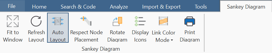
Fit to Window: When the Sankey diagram is created (concurrently with the respective tools’ table) it may display a bit too tiny in its reserved window pane. There are several options to fix this: Switch off the table view and the selection lists, maximize the project window or float the tool with the diagram. The Sankey diagram itself will not resize to the freed space automatically. Click Fit-to Window to fit the current diagram to the available window area.
Refresh Layout: This will also move nodes to their original places if moved in the meantime. The edges will also be recalculated for best entanglement. This option can also be activated by double-clicking the diagrams background.
Auto Layout: This option is activated by default. It will instantly recompute the diagram’s layout if:
- Nodes are moved
- Nodes are removed
- Edges are removed
Respect Node Placement: You might not always be happy when the nodes you shifted to other locations are instantly moved back to their original locations. To prevent this, you either need to disable the Auto Layout or select Respect Node Placement.
Note, that the Respect Node Placement option will not let you place nodes to arbitrary positions but will find the nearest lane and relayout the diagram to make it nice looking again. Shortcut: Double-click the diagram background while pressing the left Shift key.
Rotate Diagram: Sometimes the horizontal left-to-right layout may not always give the most optimal visualization of your data (depending on available screen space, monitor size). Click this button to toggle between a vertical (top-down) and the original horizontal layout. Shortcut: Double-click the diagram background while pressing the left Ctrl-key.
Display Icons: This display the entities type icons preceding the labels. This makes most sense when the diagram contains multiple types of entities as in the Code Document Table. By default, this option is not activated.
Link Color Mode: The coloring of the links and edges between the nodes can be set to:
-
Use the color of the source node, either the user provided color for codes, or the type dependent color of the entities.
-
Use the color of the target node
-
Use a color gradient starting with the source and ending with the target color. This is the default. It makes tracking the endpoint of an edge quite comfortable. Shortcut: Double-click the diagram background while pressing the left Alt key.
-
None: Use a gray shade independent of any node coloring.
Short-cut: If you double-click on an edge while pressing the left Alt-key, you switch between the different color modes.
Print Diagram: Creates an output of the current diagram respecting both the selected background, and the visual selection state of both nodes and edges. The printout will not contain any quotations.
Printing can also create high quality PDFs if an appropriate printer driver is installed.
Miscellaneous
The diagram is integrated into the table tools and responds to certain options:
-
Compress, that is removing empty rows or columns, will remove corresponding elements in the diagram.
-
Clustering may reduce the number of co-occurrences and thus affects the size of edges in the diagram.
-
Swapping rows and columns reverts the original layout by 180°.
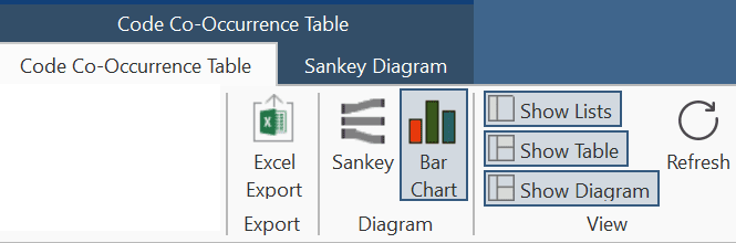
Bar Chart
To visualize the table as bar chart, click on Bar Chart in the Diagram section of the ribbon.
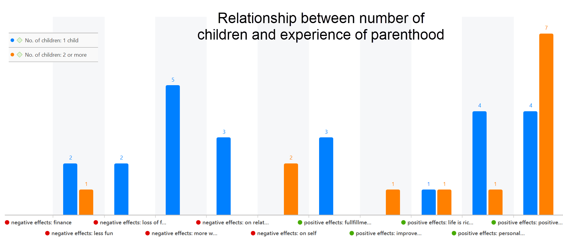
 For the visualization as bar chart, it is often preferable to change the code colors. You may also want to switch around the rows and the columns. You find this option in the ribbon of the Code Co-occurrence Table.
To create the table below, the color of the two subcodes '1 child' and '2 or more' were changed to orange and blue. The result is of course the same - for people with two or more children the table shifts significantly to the right towards the codes coding the positive experiences. Or to put it the other way around, for those with one child, both positive and negative experiences are reported with somewhat more emphasis on the negative experiences.
 If we change the rows and the columns, so that the number of children is on the x-axis, we get a more meaningful graph if we change the code colors for the subcodes of positive and negative effects. The negative effects have colors ranging from yellow to pink, the colors for positive effect range from green to blue.
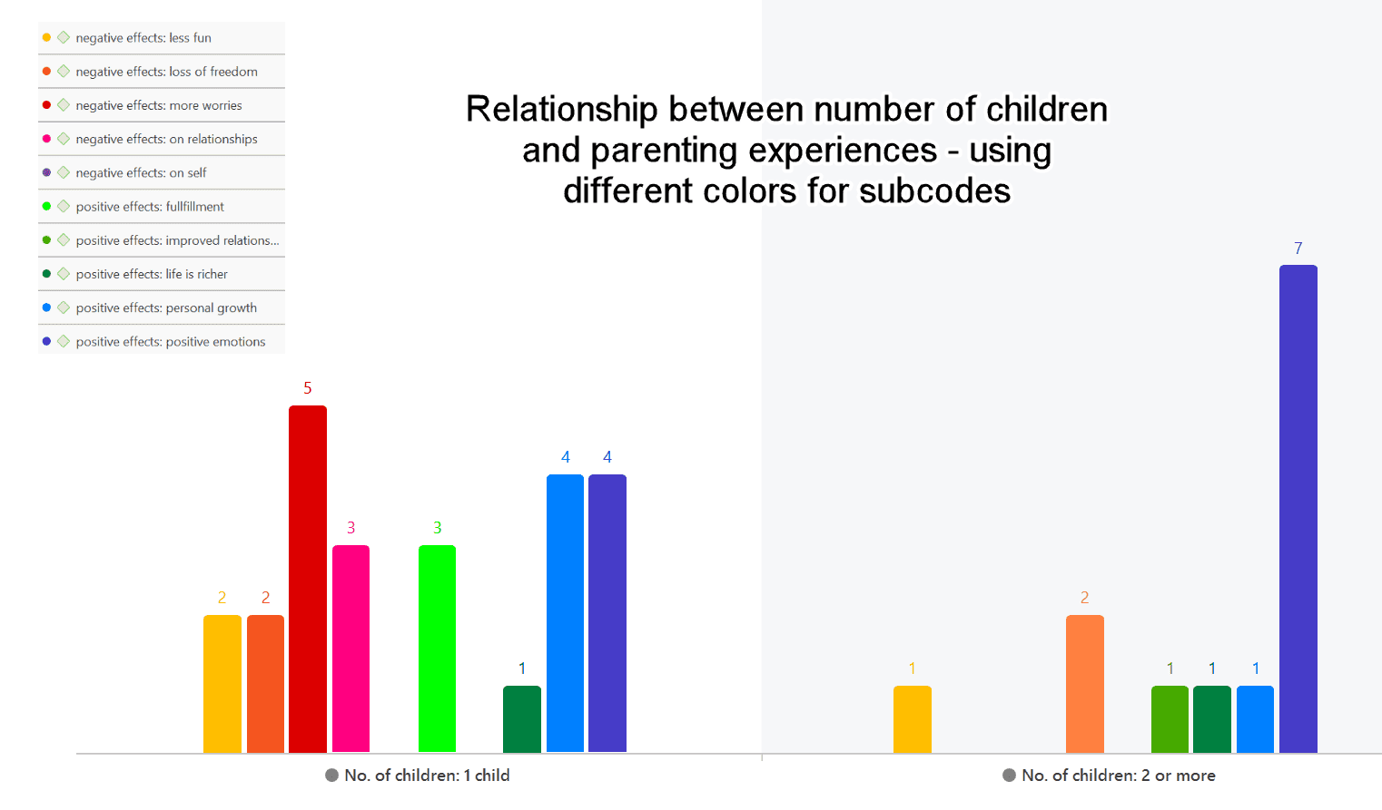
There is currently no legend. The one you see in the images are copy & pasted screenshots. Also, the code colours have to be changed manually. For a more convenient work with the graphics there will be further options in future updates.